Go to http://somafm.com and listen to “Boot Liquor” radio!
Y’all have a good day!
Go to http://somafm.com and listen to “Boot Liquor” radio!
Y’all have a good day!

This work is licensed under a Creative Commons Attribution-ShareAlike 4.0 International License.
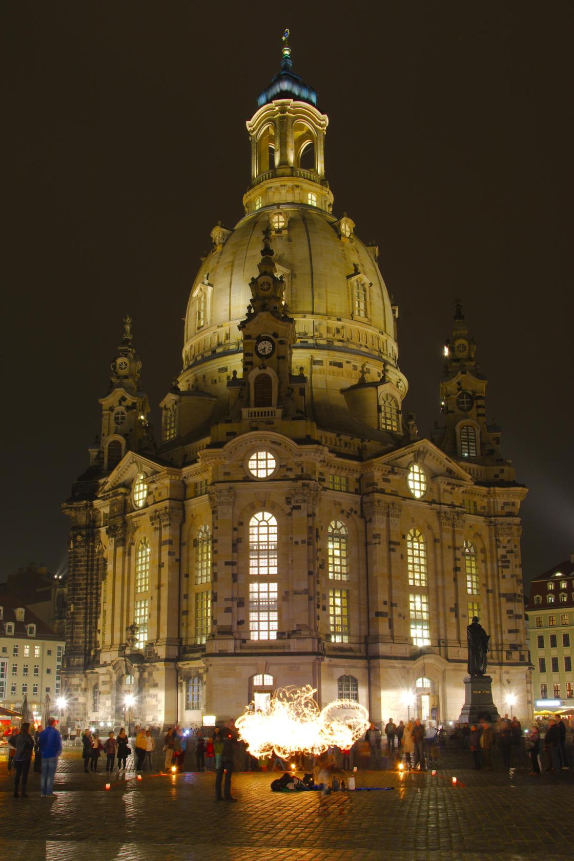
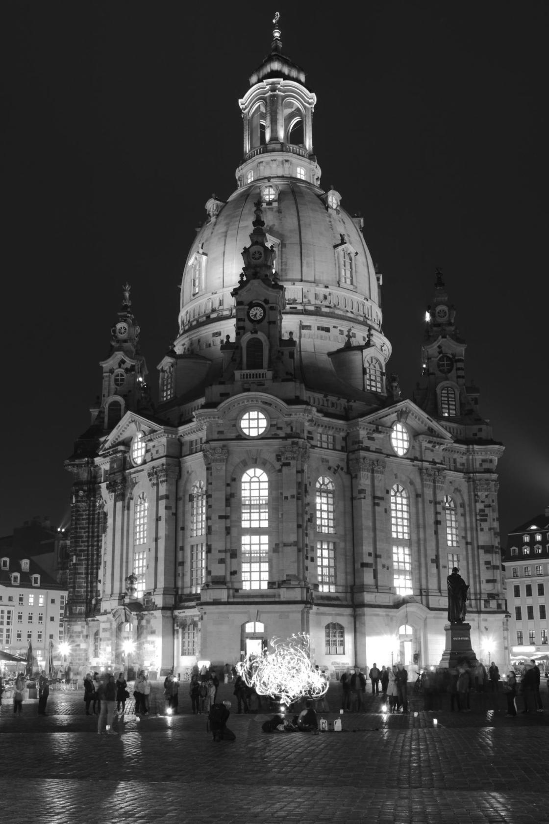
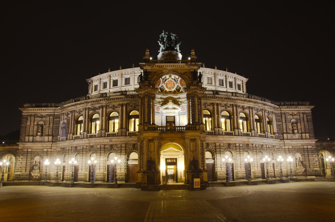
Recently I acquired a Nikon D7100 DSLR. With this nice camera I was able to shoot in RAW (uncompressed and unprocessed photo file format) and I needed a good editing tool for those files. Since these files come unprocessed from the camera’s sensor, I need to do the photo editing like setting the contrast, color tones, sharpness etc. on my computer. As you might guess there aren’t many programs for photo editing on Linux on the market. Some of them are open source and some proprietary. However the choice is very limited.
For my photography workflow I need programs for things like
Organizing & minimal editing
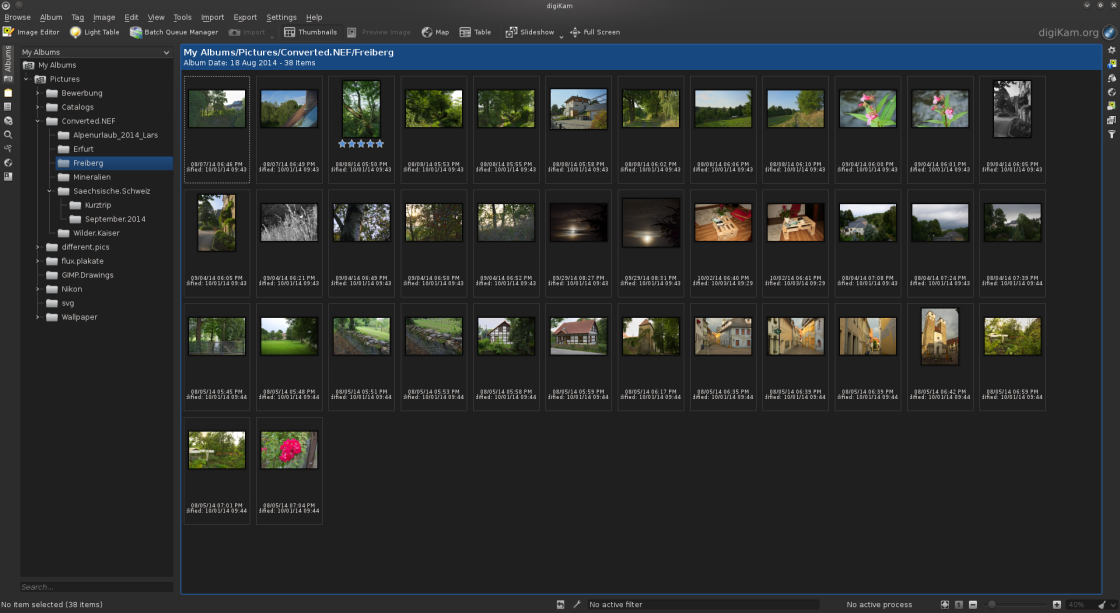
An open source tool for organizing photos is KDE’s digiKam. I can create albums for sets of photos, rate them and do some editing, resizing as well. I can look at pictures taken at different locations (GPS map) or dates (calendar) and the program sorts them accordingly. digiKam not only lets me view JPG but also RAW files and with this program I can easily download the pictures from my camera.
Editing RAW’s
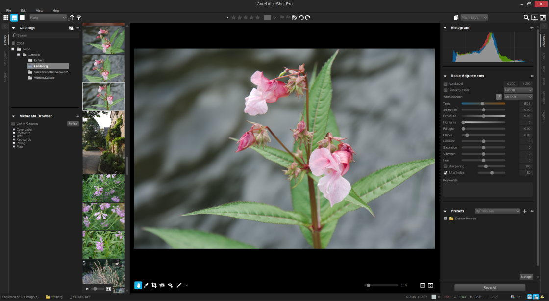
For RAW editing I currently use two. One is the proprietary program “Corel AfterShot Pro 2” and the second one is the open source alternative “RawTherapee”. Both have many features for editing RAW and I get really great pictures with both of them. Also a rating and sorting / tagging feature can be found in both.
“Corel AfterShot Pro 2” may have some better sorting mechanisms and algorithms for editing sharpness of the photo. However someone can also create awesome shots with “RawTherapee”. I for example find the queue manager better in the open source program. However I like them both and since “Corel AfterShot Pro 2” is also available on Linux for around 50€ I can and will use them both. Another thing is that a HDR editing feature will come out soon. This gives me a program for sorting, editing and creating HDR’s all in one.
Creating HDR’s
A real HDR is created by stacking several photos of different exposures together to create a final photo with high contrasts in shadow as well as bright areas. An open source tool for that purpose is “Luminance HDR”. I don’t have really used this program because it used a lot of RAM to stack a few pictures together. I have 8 GB of RAM, which should be sufficient though. Maybe “Luminance HDR” works on your machine better :)
Therefor I will be waiting for Corel to release the update for creating HDR’s in “AfterShot Pro 2”, because I didn’t find a better solution than “Luminance HDR” on Linux yet.
OpenFOAM is an open-source CFD (computational fluid dynamics) toolbox, which you can use on your GNU/Linux machine. To get started with OpenFOAM you can read the documentation on the website and/or run tutorial cases. For every solver there are several tutorial cases which you can run on your PC. However you probably need to know more to set up your own simulations. First of all some general information on CFD. Every Simulation consists of several steps, you have to go through, before you can view your results. These steps are:
Preprocessing includes building the CAD geometry and deciding on the boundary conditions (BC’s). It means that the CAD geometry will be meshed, which means the surface of the CAD geometry will be used to create an underlying grid, representing your original geometry features. On this grid/mesh the solver calculates the values for the several transport equations (mass, motion and energy). This is meant by the term solving. With the mesh the equations of motion, energy and mass are solved on each grid point. Meaning the more grid points one has (a finer the mesh) the longer it takes to solve the simulation, but also a finer mesh may result in a more accurate solution. Problem is: An accurate solution depends on your mesh (quality and size), algorithms, included simplifications (make your case solvable but inaccurate because you just can’t account for everything).
One example of such a simplification is turbulence. This is a really complex physical process where eddies (velocity fluctuations) of any size occur in a flow field. The physics behind it are not yet fully understood and therefor mathematical models are necessary to simplify this process. Since these eddies range from really small (microscopic) to really large (macroscopic) the requirements on the mesh are extreme to simulate very tiny eddies (DNS – Direct Numerical Simulation). One can account only a range of eddies by applying a filter (LES – Large Eddy Simulation). It is also possible, since turbulence is a highly transient process, to average over time (RANS – Reynolds Averaged Navier Stokes) and therefor reduce the equation of motion by several unknowns, the velocity fluctuations. But enough from turbulence … for now :)
After the solving of the problem you get values for p, U, T (depending on the solver) …
p: Pressure
U: Velocity
T: Temperature
on every grid point. In Postprocessing these values can now be plotted as scalar fields (p, T) or vector fields (U). For postprocessing the tool “paraFoam” (which is Paraview) is included in every OpenFOAM installation. It lets you process the data from the time folders (0, 5, 10 etc.) very easily. Contour plots, surface plots of scalar or vector fields, vector plots (glyphs), slices … you name it. Many filters will help you sort your data, clip and modify data.
There are 3 default folders in every case folder:
The folder “0” includes all boundary conditions or initial conditions for your simulation. In “constant” are the properties of the fluids, solids, porous media stored as well as the value of the gravitational vector “g”. Inside this folder you’ll find another folder “polyMesh” which includes the data of your mesh (points, faces etc.). In “system” the properties of the solution algorithms (fvSolution, fvSchemes) and properties of the simulation are stored in the “controlDict”.
(to be continued)